There’s a lot to like about the Intel OpenBot, which I wrote about last month. Since that post, the Intel team has continued to update the software and I’m hopeful that some of the biggest pain points, especially the clunky training pipeline (which, incredibly, required recompiling the Android app each time) will be addressed with cloud training. [Update 1/22/21: With the 0.2 release, Intel has indeed addressed these issues and now have a web-based way to handle the training data and models, including pushing a new model to the phone without the need for a recompile. Bravo!]
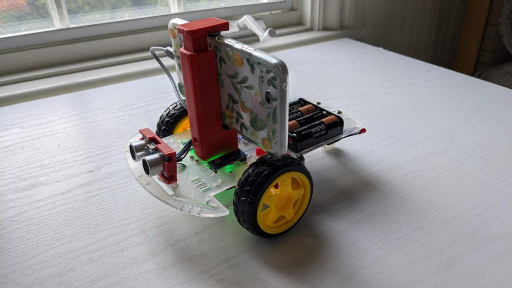
On the hardware side, I could see an easy way to improve upon Intel’s design, which required too much 3D printing and used a ungainly 4 wheel-drive design that was very difficult to turn. There are plenty of very cheap 2WD chassis on Amazon, which use a trailing castor wheel for balance and turning nimbleness. 2WD is cheaper, better, easier and to be honest, Intel should have used it to begin with.
So I modified Intel’s design for that, and this post will show you how you can do the same.
First, buy a 2WD chassis from Amazon. There are loads of them, almost all exactly alike, but here’s the one I got ($12.99)
If you don’t have a 3D printer, you can buy a car phone mount and use that instead.
The only changes you’ll need to make to Intel’s instructions are to drill a few holes in the chassis to mount the phone holder. The plexiglass used in the Amazon kits is brittle, so I suggest cutting a little plywood or anything else you’ve got that’s flat and thin to spread the load of the phone holder a bit wider so as not to crack the plexiglass.
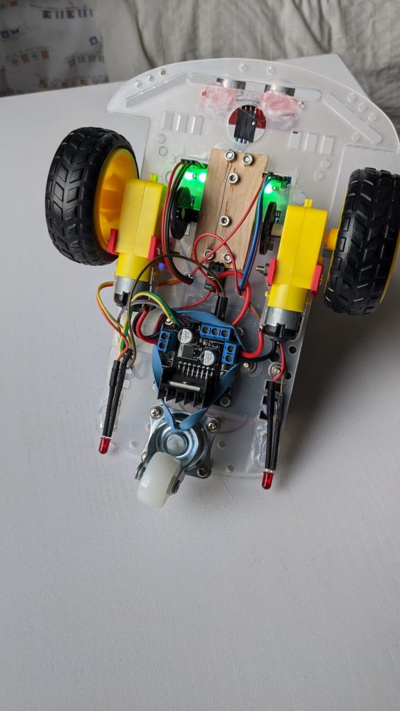
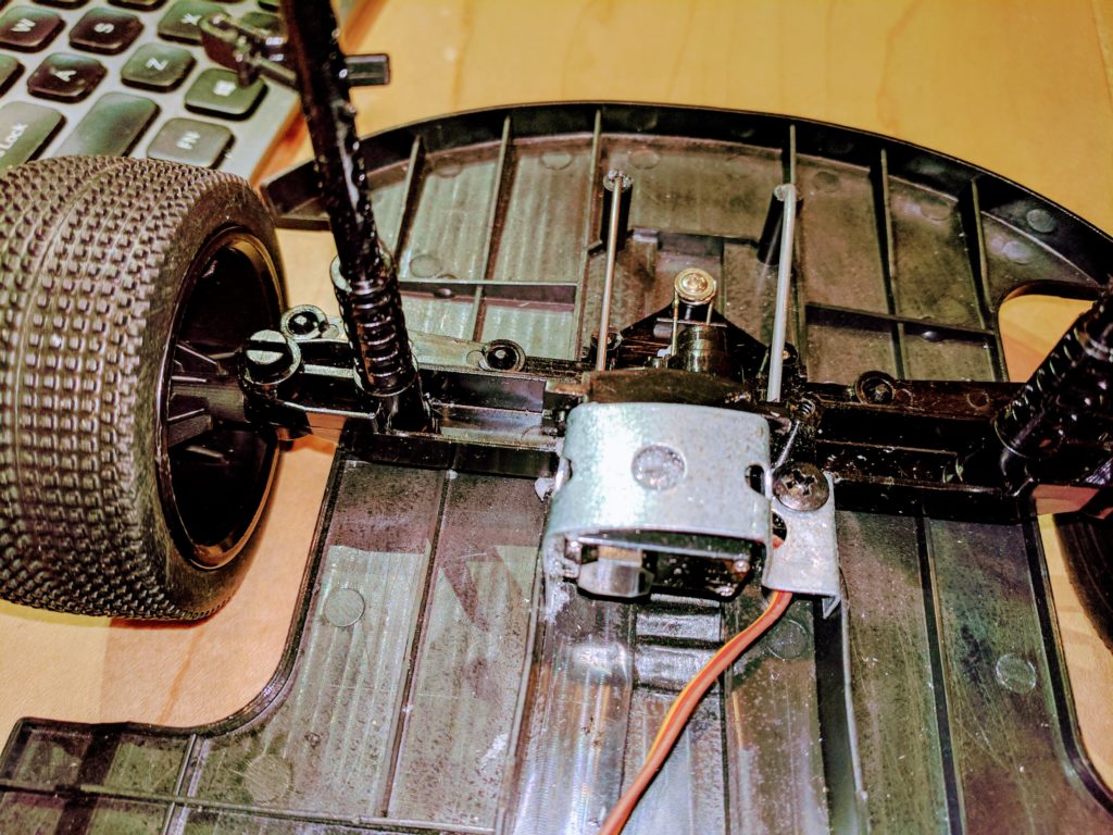
You can see how I used a little plywood to do that below
You will also have to expand some of the slots in the plexiglass chassis to fit the encoders. If you have a Dremel tool, use a cutoff wheel for that. If not, carefully use a drill to make a line of holes.
Everything else is as per the Intel instructions — the software works identically. I think the three-wheel bot works a bit better if the castor wheel is “spring-loaded” to return to center, so I drilled in a hole for a screw in the castor base and wrapped a rubber band around it to help snap the wheel back to center as shown above, but this is optional and I’m not sure if it matters all that much. All the other fancy stuff, like the “turn signal” LEDs and the ultrasonic sensor, are also optional (if you want to 3D print a mount for the sonar sensor, this is the one I used and I just hot-glued it on).
I’d recommend putting the Arduino Nano on the small solderless breadboard, which makes adding all jumper wires (especially the ground and V+ ones) so much easier. You can see that below.
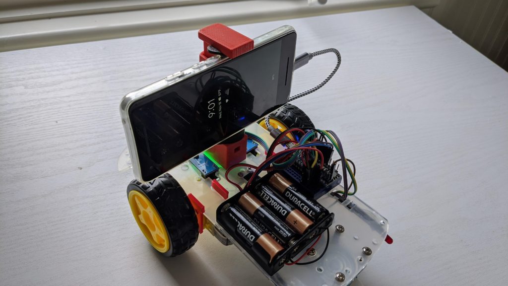
Here it is (below) running in manual mode in our house. The 4 AA batteries work pretty much the same as the more expensive rechargeable ones Intel recommends. But getting rid of two motors is the key — the 2WD is so much more maneuverable than the 4WD version and just as fast! Honestly, I think it’s better all around — cheaper, easier and more nimble. OpenBot with 2WD chassis – YouTube
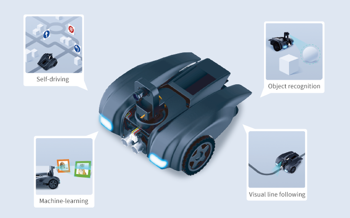
tl;dr: The Tinkergen MARK ($199) is my new favorite starter robocar. It’s got everything — computer vision, deep learning, sensors — and a great IDE and set of guides that make it all easy and fun.
Getting a robocar design for first-time users right is a tricky balance. It should be like a great videogame — easy to pick up, but challenging to master. Too many kits get it wrong one way or another. They’re either too basic and only do Arduino-level stuff like line-following or obstacle avoidance with a sonar sensor, or they’re too complex and require all sorts of toolchain setups and training to do anything useful at all.
In this post, I list three that do it best — Zumi, MARK, and the Waveshare Piracer. Of those, the Piracer is really meant for more advanced users who want to race outdoors and are comfortable with Python and Linux command lines — it really only makes the hardware side of the equation easier than a fully DIY setup. Zumi is adorable but limited to the Jupyter programming environment running via a webserver on its own RaspberryPi Zero, which can be a little intimidating (and slow).
But the Tinkergen MARK gets the balance just right. Like the others, it comes as a very easy to assemble kit (it takes about 20 minutes to screw the various parts together and plug in the wires). Like Zumi, it starts with simple motion control, obstacle detection and line following, but it also as some more advanced functions like a two-axis gimbal for its camera and the ability to control other actuators. It also has a built-in screen on the back so you can see what the camera is seeing, with an overlay of how the computer vision is interpreting the scene.
Where MARK really shines is the learning curve from basic motion to proper computer vision and machine learning. This is thanks to its web-based IDE and tutorial environment.
Like a lot of other educational robotics kits designed for students, it defaults to a visual programming environment that looks like Scratch, although you can click an icon at the top and it switches to Python.
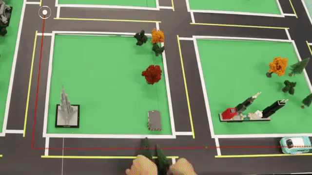
Videos and guides are integrated into the web interface and there are a series of courses that you can run through at your own pace. There is a full autonomous driving course that starts with simple lane-keeping and goes all the way to traffic signs and navigation in a city-street like environement.
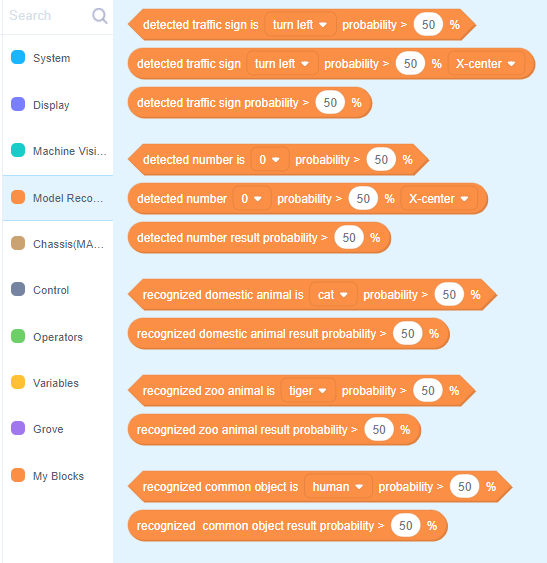
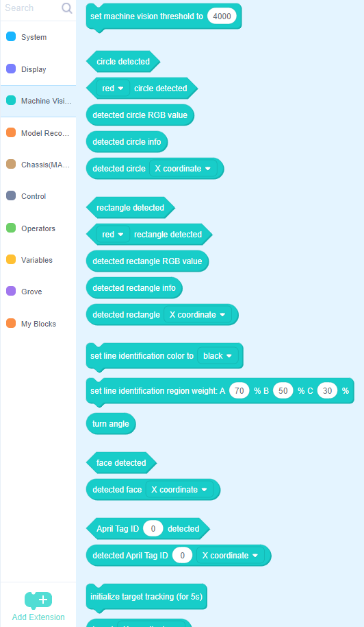
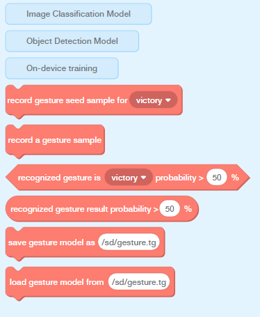
Where MARK really shines is in the number of built-in computer vision and deep learning functions. Pre-trained networks include recognizing traffic signs, numbers, animals and other common objects:
Built-in computer vision modules include shapes, colors, lines, faces, Apriltags and targets. Also supported is both visual line following (using the camera) or sensor line following using the IR emitter/receiver pairs on the bottom of the car.
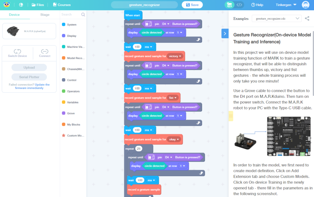
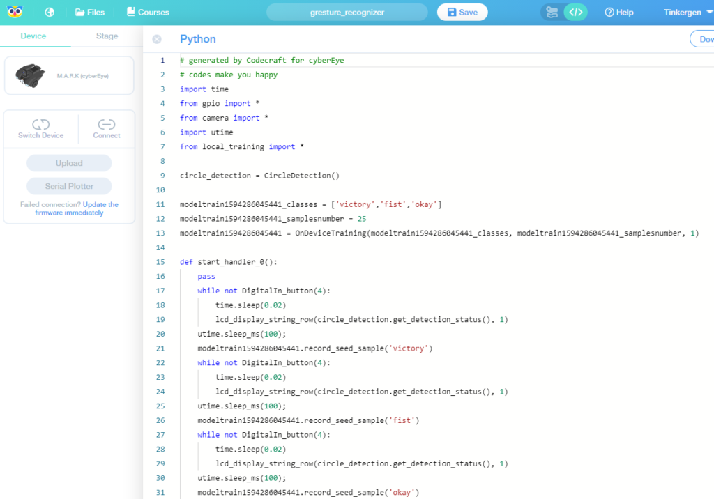
In addition, you can can train it to identify new objects and gestures by recording images on the device and then training a deep learning network on your PC, or even training on the MARK itself for simpler objects.
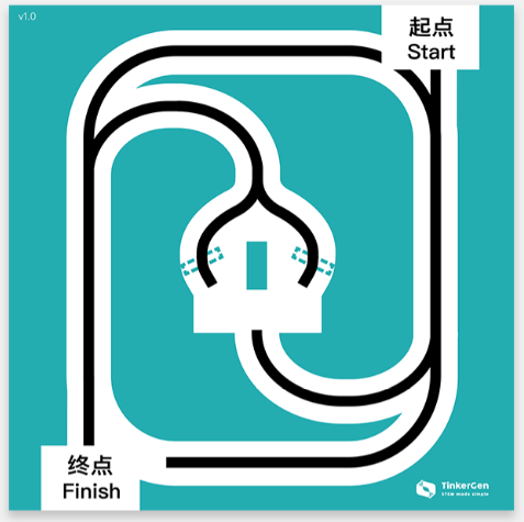
I got the track mat as well with the kit, which is the right size and contrast to dial in your code so it performs well. Recommended.
In short, this is the best robocar kit I’ve tried — it’s got very polished hardware and software, a surprisingly powerful set of features and great tutorials. Plus it looks great and is fun to use, in large part due to the screen at the top that shows you what the car is seeing. A great Holiday present for kids and adults alike — you won’t find a better computer vision and machine learning experimentation package easier to use than this.
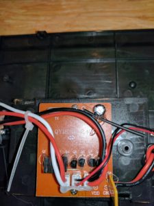
Intel has released an open source robocar called OpenBot that uses any Android phone running deep-learning code to do autonomous driving, including navigating in halls or on a track or following a person. The key bit here is the open source Intel Android app, which does all the hard work; the rest of the car is just a basic Arduino and standard motors+chassis.
To be honest, I had not realized that it was so easy to get an Android phone to talk to an Arduino — it turns out that all you need is an OTG (USB Type C to USB Micro or Mini) cable for them to talk serial with each other. (This is the one I used for Arduinos that have a USB Micro connector.) Sadly this is not possible with iOS, because Apple restricts hardware access to the phone/tablet unless you have a special licence/key that is only given out to approved hardware.
The custom Intel chassis design is very neat, but it does require a lot of 3D printing (a few days’ worth). I don’t really understand why they didn’t just use a standard kit that you can buy on Amazon instead and just have the user 3D print or otherwise make or buy a phone holder, since everything else is totally off the shelf. Given how standard the chassis parts are, it would be cheaper and easier to use a standard kit.
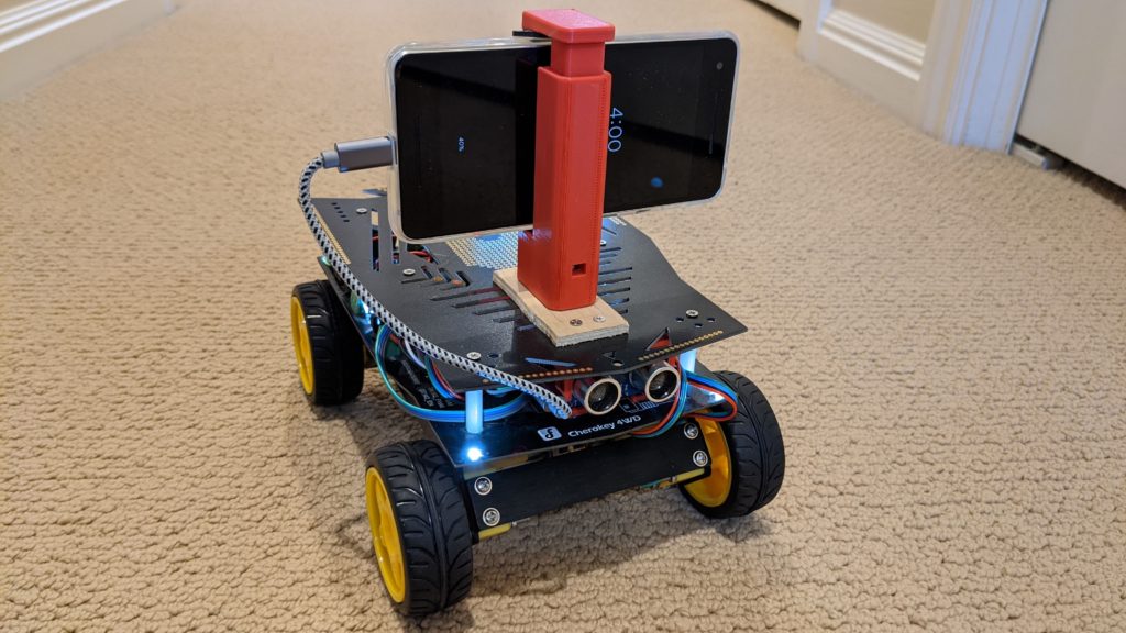
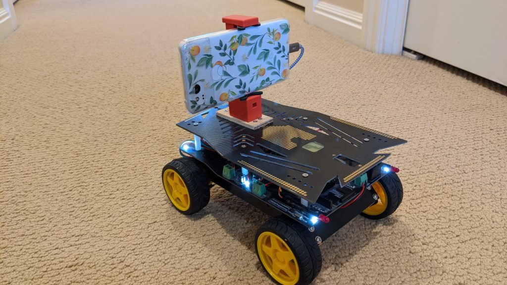
I ended up using a chassis I had already, which is the DFRobot Cherokey car. It’s slightly overkill, since it has all sorts of wireless communications options built in, including bluetooth and and Xbee socket, that I didn’t need, but it’s just evidence that you can use pretty much any “differential drive” (steering is done by running motors on the left and right at different speeds) chassis you have handy. Basically any car that uses an Arduino will work with a little tweaking.
I took a few other liberties. I had some motors that had built-in quadrature encoders, which I prefer to the cheap optical encoders Intel recommended, so I had to modify the code a bit for them and that meant changing a few pin mappings. (You can see my modified code here.). But otherwise it’s pretty much as Intel intended, complete with sonar sensor and cute turn signals at the back.
So how does it work? Well, for the easy stuff, great. It does person following right out of the box, so that’s a good test if your bot is working right. But the point is to do some training of your own. For that, Intel has you drive manually with a bluetooth game controller, such as a PS4 controller, to gather data for training on your laptop/PC. That’s what I did, although Intel doesn’t tell you how to pair the controller with your Android phone ( (updated) the answer: press the controller PS and the Share button until the light starts flashing blue fast. Then you you should be able to see it in your Android Bluetooth settings “pair new device” list. More details here).
But for the real AI stuff, which is learning and training new behavior, it’s still pretty clunky. Like DonkeyCar, it uses “behavioral cloning”, which is to say that the process is to drive it manually around a course with the PS4 controller, logging all the data (camera and controller inputs) on your phone, then transfer a big zip file of that data to your PC, which you run a Jupyter notebook inside a Conda environment that uses TensorFlow to train a network on that data. Then you have to replace one of the files in the Android app source code with this new model and recompile the Android app around that. After that, it should be able to autonomously drive around that same course the way you did.
Two problems with this: first, I couldn’t get the Jupyter notebook to work properly on my data and experienced a whole host a problems, some of which were my fault and some were bugs in the code. The good news is that the Intel team is very responsive to issue reports on Github and I’m sure we’ll get those sorted out, ideally leading to code improvements that will spare later users these pain points. But overall, the data gathering and training process is still way too clunky and prone to errors, which reflects the early beta nature of the project.
Second, it’s crazy that I have to recompile the Android app every time I train a new environment. We don’t need to do that with DonkeyCar, and we shouldn’t have to do that with OpenBot, either. Like DonkeyCar, the OpenBot app should be able to select and load any pretrained model. It already allows you to select from three (person following and autopilot) out of the box, so it’s clearly set up for that. So I’m confused why I can’t just copy a new model to a directory on my phone and select that from within the app, rather than recompiling the whole app.
Perhaps I’m missing something, but until I can get the Jupyter notebook to work it will just have to be a head-scratcher…
There are a load of great DIY projects you can find on this site and elsewhere, such as the OpenMV minimum racer and Donkeycar. But if you’re not feeling like you’re ready for a DIY build here are a few almost ready-to-run robocars that come pretty much set up out of the box.
My reviews of all three are below, but the short form is that unless you want to race outdoors, the Tinkergen MARK is the way to go.
What kind of car should you make autonomous? They all look the same! There are some amazing deals out there! How to choose??
I’m going to make it easy for you. Look for this:
What’s that? It’s a standard RC connector, which will allow you to connect steering and throttle to standard computer board (RaspberryPi, Arduino, etc). If you see that in car, it’s easily converted into autonomy. (Here’s a list of cars that will work great)
If you don’t see that, what you’ve got is CRAZY TOY STUFF. Don’t buy it!
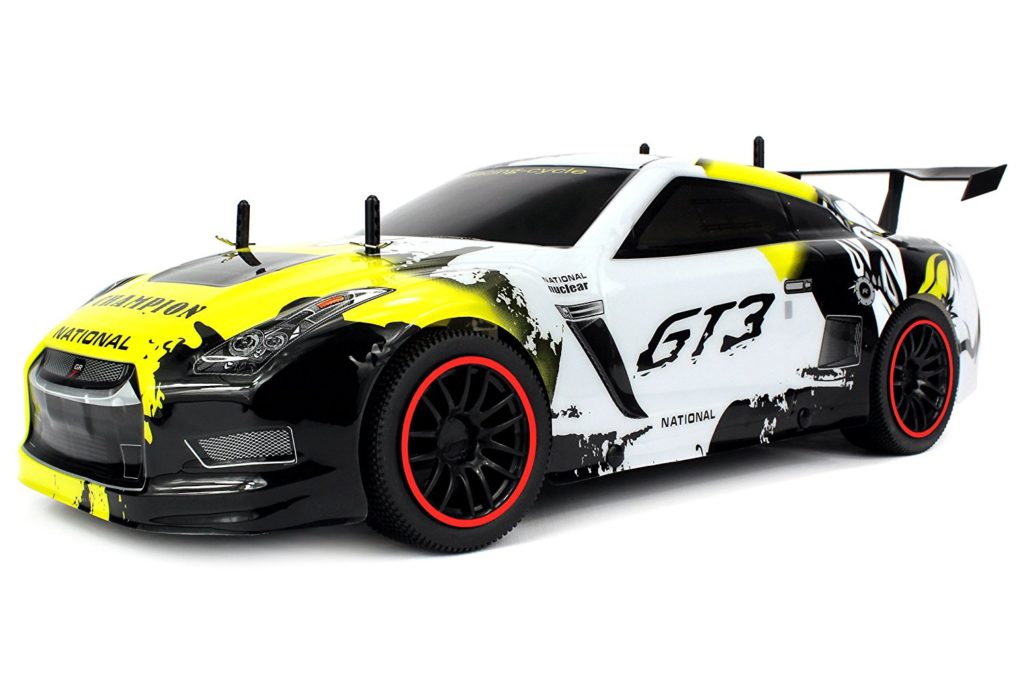
But let’s say you already have, because you saw this cool looking car on Amazon (picture above) for just $49
By the looks of it, it’s got all this great stuff:
HIGH PERFORMANCE MOTOR: Can Reach Speeds of Approximately Up to 15 MPH ·
RECHARGEABLE LITHIUM BATTERY: High Performance Lithium-Ion Battery · Full Function Pro Steering (Go Forward and Backward, Turn Left and Right) · Adjustable Front Wheel Alignment
PRO 2.4GHz RC SYSTEM: Uninterrupted, Interference-Free Driving · Race Multiple Cars at the Same Time
Requires 6.4v 500mAh Lithium-Ion Battery to run (Included) Remote Control requires 9v Battery to run (Included)
BIG 1:10 SCALE: Measures At a Foot and a Half Long (18″) · Black Wheels with Premium, Semi-Pneumatic, Rubber Grip Tires · Interchangeable, Lightweight Lexan Body Shell with Metal Body Pins and Rear Racing Spoiler · Approximate Car Dimensions, Length: 18″ Width: 8″ Height: 5″
But is it good for autonomy? Absolutely not. Here’s why:
When you get it, it looks fine:
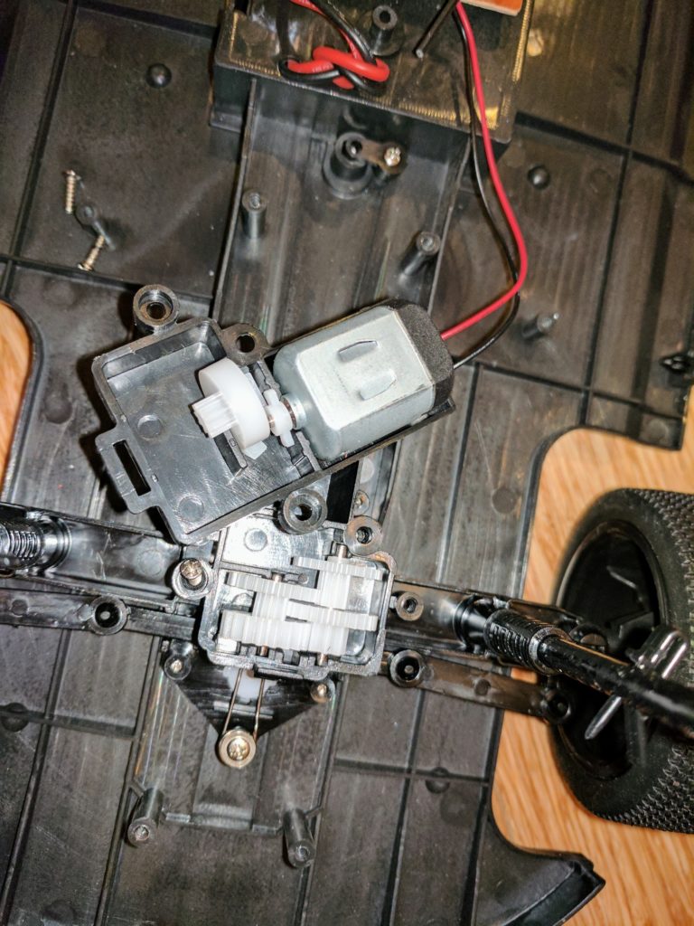
But what’s inside? Erk. Almost nothing:
That’s not servo-driven steering! 🙁 Instead, it’s some weird thing with a motor, some gears and a spring:
How about the RC? Yikes. Whatever this thing is, you can’t use it (it’s actually an integrated cheap-ass radio and motor controller — at any rate there’s no way to connect a computer to it)
So total write-off? Not quite.
Here’s what you have to do to make it usable:
First, you’ve to to put in a proper steering servo. Rip out the toy stuff, and put in a servo with metal gears (this one is good). Strap it in solidly, like I have with a metal strap here:
Now you have to put in a proper RC-style motor controller and power supply. These cheap cars have brushed motors, not brushless ones, so you need to get a brushed ESC. This one is fine, and like most of them has a power supply (called a BEC, or battery elimination circuit), too.
Now you can put in your RaspberryPi and all the other good stuff, including a proper LiPo battery (not that tiny thing that came with it).
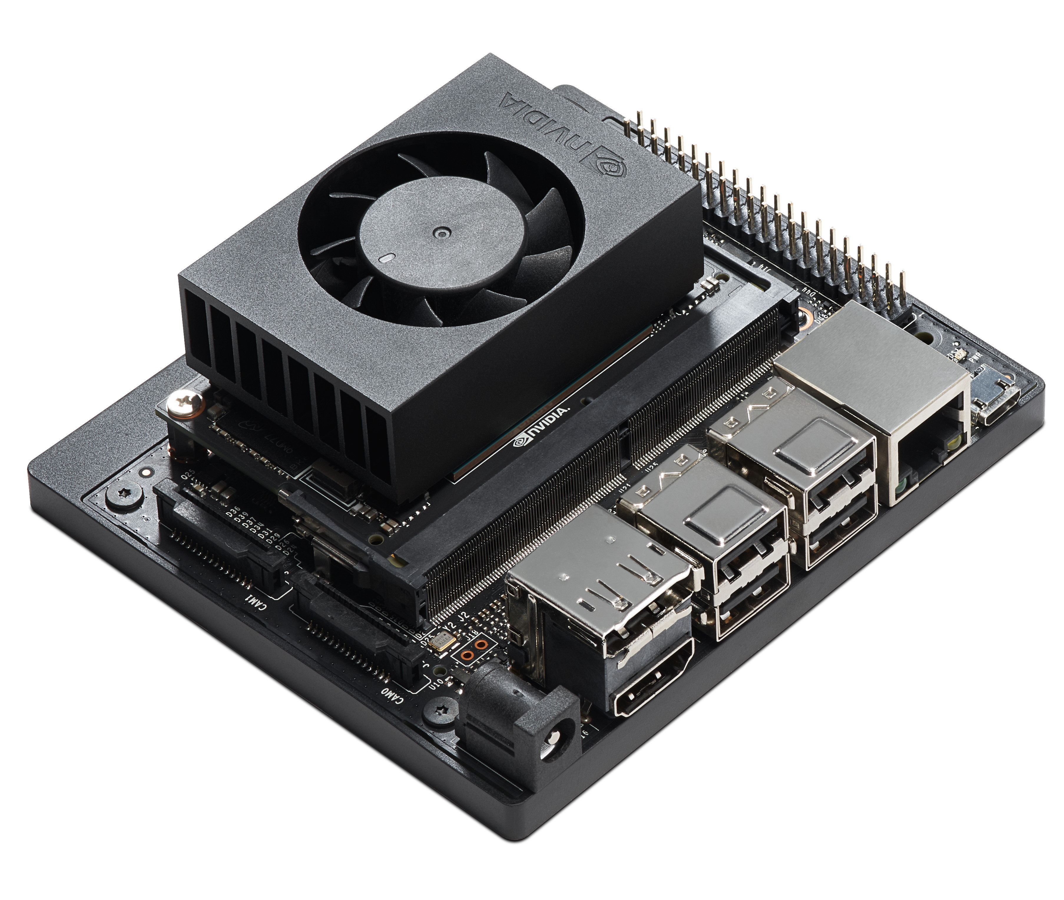
It’s now been a couple weeks since Nvidia released its new Jetson Xavier NX board, a $399 big brother to the Jetson Nano (and successor to the TX2) with 5-10 times the compute performance of the Nano (and 10-15x the performance of a RaspberryPi 4) along with twice as much memory (8 Gb). It comes with a similar carrier board as the Nano, with the same Raspberry Pi GPIO pins, but includes built-in Wifi/BT and a SSD card slot, which is a big improvement over the Nano.
How well does it suit DIY Robocars such as Donkeycar? Well, there are pluses and minuses:
Pros:
All that computing power means that you run deeper learning models with multiple camera at full resolution. You can’t beat it for performance.
It also means that you can do your training on-car, rather than having to export to AWS or your laptop
Built-in wifi is great
Same price but smaller and way more powerful than a TX2.
Cons:
Four times the price of Nano
The native carrier board for the Jetson NX runs at 12-19v, as opposed the Nano, which runs at 5v. That means that the regular batteries and power supplies we use with most cars that use Raspberry Pi or Nano won’t work. You have two options:
2) Use a Nano’s carrier board if you have one. But you can’t use just any one! The NX will only work with the second-generation Nano carrier board, the one with two camera inputs (it’s called B-01)
When it shipped, the NX had the wrong I2C bus for the RPi-style GPIO pins (it used the bus numbers from the older TX2 board rather than the Nano, which is odd because it shares a form factor with the Nano). After I brought this to Nvidia’s attention they said they would release a utility that allows you to remap the I2C bus/pins. Until then, RPi I2C peripherals won’t work unless they allow you to reset their bus to #8 (as opposed to the default #1). Alternatively, if your I2C peripheral has wires to connect to the pins (as opposed to a fixed header) you can use the NX’s pins 27 and 28 rather than the usual 3 and 5, and that will work on Bus 1
I’ve managed to set up the Donkey framework on the Xavier NX and there were a few issues, mostly involving that fact that it ships with the new Jetpack 4.4, which requires newer version of TensorFlow than the standard Donkey setup. The Donkey docs and installation scripts are being updated to address that and I’m hoping that by the time you read this the setup should be seamless and automatic. In the meantime, you can use these installation steps and it should work. You can also get some debugging tips here.
I’ll also be trying it with the new Nvidia Isaac robotic development system. Although the previous version of Isaac didn’t work with the Xavier NX, version 2020.1 just came out so fingers crossed this works out of the box.
There are so many cool sensors and embedded processors coming out of China these days! The latest is the amazing HuskyLens, which is a combination of a powerful AI/computer vision processor, a camera and a screen — for just $45. HuskyLens comes with a host of CV/AI functions pre-programmed and a simple interface of a scroll wheel and a button to choose between them and change their parameters.
To test its suitability for DIY Robocars, I swapped it in on my regular test car, replacing an OpenMV camera. I used the same Teensy-based board I designed for the OpenMV to interface with a RC controller and the car’s motor controller and steering servo. But because the HuskyLens can’t be directly programmed (you’re limited to the built-in CV/AI functions) I used it just for the line-following function and programmed the rest of the car behavior (PID steering, etc) on the Teensy. You can find my code here.
As you can see from the video above, it works great for line following.
Advantages of the HuskyLens include:
It’s super fast. I’m getting 300+ FPS for line detection. That’s 5-10x the speed of OpenMV (but with some limitations as discussed below)
Very easy to interface with an Arduino or Teensy. The HuskyLens comes with a cable that you can plug into the Arduino/Teensy and an Arduino library to make it easy to read the data.
The built-in screen is terrific, not only as a UI but to get real-time feedback on how the camera is handling a scene without having to plug it into a PC.
Easy to adjust for different lighting and line colors
Built-in neural network AI programs that make it easy to do object detection, color detection, tags, faces and gestures. Just look at what you want to track and press the button.
Compared to the OpenMV, some disadvantages of HuskyCam include:
You can’t change the camera or lens. So no fisheye lens option to give it a wider angle of view
You can’t directly program it. So no fancy tricks like perspective correction and tracking two different line colors at the same time
You’ll have to pair it with an Arduino or Teensy to do any proper work like reading RC or driving servos (OpenMV, in contrast, has add-on boards that do those things directly)
It consumes about twice the power of OpenMV (240ma) so you may need a beefier power supply than simple the BEC output from your car’s speed controller. To avoid brownouts, I decided not to use the car’s regular motor controller’s output to power the system and used a cheap switching power supply instead.
If you want to do a similar experiment, here are some tips on my setup:
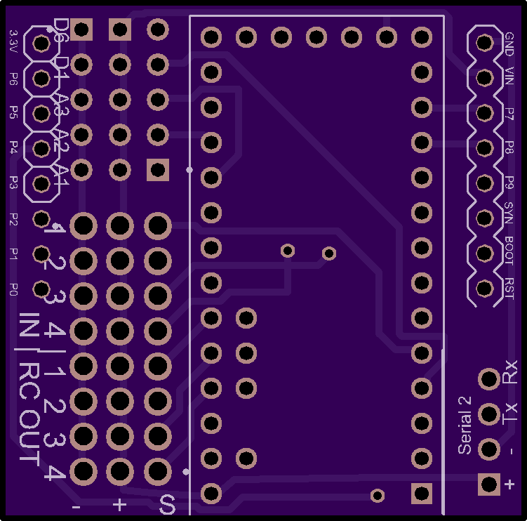
You can order my Teensy RC PCB, to make the connections easier, from OSHPark here. It also works with OpenMV.
After you solder in the Teensy with header pins, solder in a 3-pin header for RC IN 1,2,3 and RC OUT 1 and 2. You’ll connect your RC receiver’s channels 1 and 2 to RC IN 1 and 2 and whichever channel you want to use to switch from RC to auto modes to RC IN 3. Connect the steering servo to RC Out 1 and the motor controller to RC Out 2. If you’re using a separate power supply, you can plug that into any spare RC in or out pins
Also solder a 4-pin connect to Serial 2. Your HuskyLens will plug into that. Connect the HuskyLens “T” wire to the Rx and “R” wire to the Tx, and + and – to the corresponding pins.
Software:
My code should pretty much work out of the box on a Teensy with the above PCB. You’ll need to add the HuskyLens library and the AutoPID library to your Arduino IDE before compiling.
It assume that you’re using a RC controller and you have a channel assigned (plugged into RC IN 3) for selecting between RC and HuskyLens controlled modes. If you don’t want to use a RC controller, set boolean Use_RC = true; to false
It does a kinda cool thing of blending the slope of the line with its left-right offset from center. Both require the car to turn to get back on line.
If you’re using RC, the throttle is controlled manually with RC in both RC and auto modes. If not, you can change it by modifying this line: const int cruise_speed = 1600;. 1500 is stopped; less than that is backwards and more than that (up to 2000) is forwards at the speed you select.
It uses a PID controller. Feel free to change the settings, which are KP, KI and KD, if you’d like to tune it
On your HuskyLens, use the scroll wheel to get to General Settings and change the Protocol/Serial Baud Rate to 115200.
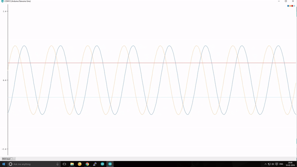
If you use Arduino, perhaps to handle the lower-level driving work of your DIY Robocar, you may have noticed the Serial Plotter tool, which is an easy way to graph data coming off your Arduino (much better than just watching numbers scroll past in the Serial Monitor).
You may have also noticed that the Arduino documentation gives no instructions on how to use it ¯\_(ツ)_/¯. You can Google around and find community tutorials, such as this one, which give you the basics. But none I’ve found are complete.
So this is an effort to make a complete guide to using the Arduino Serial Plotter, using some elements from the above linked tutorial.
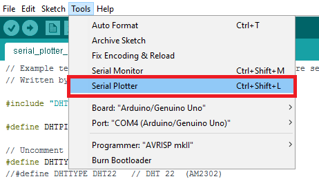
First, you can find the feature here in the Arduino IDE:
It will plot any data your Arduino is sending out in a Serial.print() or Serial.println() command. The vertical Y-axis auto adjusts itself as the value of the output increases or decreases and the X-axis is a fixed 500-point axis with each tick of the axis equal to an executed Serial.println() command. In other words the plot is updated along the X-axis every time Serial.println() is updated with a new value.
It also has some nice features:
Plotting of multiple variables, with different labels and colors for each
Can plot both integers and floats
Auto-resizes the scale (Y axis)
Supports negative value graphs
Auto-scrolls the X axis
But to make it work well, there are some tricks in how to format that data. Here’s a complete(?) list:
Keep your serial speed low. 9600 is the best for readability. Anything faster than 57600 won’t work.
Plot one variable: Just use Serial.println()
Serial.println(variable);
Plot more than one variable. Print a comma between variables using Serial.print() and use a Serial.println() for the variable at the end of the list. Each plot will have a different color.
Serial.print(variable1);
Serial.print(",");
Serial.print(variable2);
Serial.print(",");
Serial.println(last_variable); // Use Serial.println() for the last one
Plot more than one variable with different labels. The labels will be at the top, in colors matching the relevant lines. Use Serial.print() for each label. You must use a colon (and no space) after the label:
Serial.print("Sensor1:");
Serial.print(variable1);
Serial.print(",");
Serial.print("Sensor2:");
Serial.print(variable2);
Serial.print(",");
Serial.println(last_variable); // Use Serial.println() for the last one
A more efficient way to do that is to send the labels just once, to set up the plot, and then after that you can just send the data:
void setup() {
   // initialize serial communication at 9600 bits per second:
   Serial.begin(9600);
   Serial.println("var1:,var2:,var3:");
 }
void loop() {
   // read the input on analog pin 0:
   int sensorValue1 = analogRead(A1);
   int sensorValue2 = analogRead(A2);
   int sensorValue3 = analogRead(A3);
   // print out the value you read:
   Serial.print(sensorValue1);
   Serial.print(",");
   Serial.print(sensorValue2);
   Serial.print(",");
   Serial.println(sensorValue3);
   delay(1);        // delay in between reads for stability
 }
Add a ‘min’ and ‘max’ line so that you can stop the plotter from auto scaling (Thanks to Stephen in the comments for this):
Serial.println("Min:0,Max:1023");
Or if you have multiple variables to plot, and want to give them their own space:
For reasons that probably involve too much starting projects and not enough thinking about why I was starting them, I have conducted an experiment in comparing an array of ultrasonic sensors with an array of time-of-flight Lidar sensors. This post will show how to make both of them as well as their pros and cons. But [spoiler alert] at risk of losing all my readers in the first paragraph, I must reveal the result: neither are as good as a $69 2D Lidar.
Nevertheless! If you’re interested in either kind of sensors, read on. There are some good tips and lessons below.
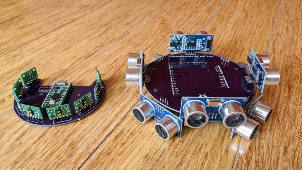
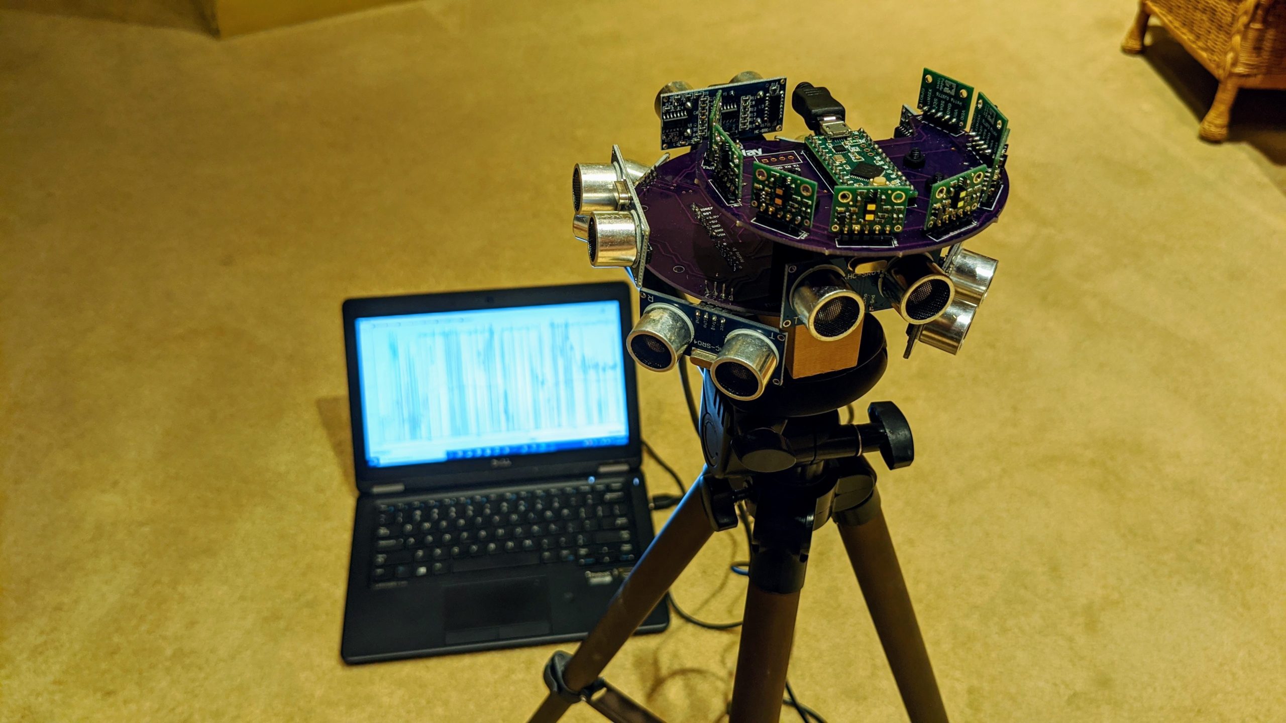
First, how this started. My inspiration was the SonicDisc project a few years ago from Dimitris Platis, which arranges eight cheap ultrasonic sensors in a disc and makes it easy to read and combine the data.
I ordered the PCBs and parts that Dimitis recommended, but got busy with other things and didn’t get around to assembling them until this year. Although I eventually did get it working, it was kind of a hassle to solder together an Arduino from the basic components, so I redesigned the board to be an Arduino shield, so it just plugs on top of a regular Arduino Uno or the like. If you want to make one like that, you can order my boards from OSH Park here. The only other parts you’ll need are eight ultrasonic sensors, which are very cheap (just $1.40 each). I modified Dimitris’ Arduino code to work as an Arduino shield; you can get my code here.
Things to note about the code: It’s scanning way faster (~1000hz) than needed and fires all the ultrasonic sensors at the same time, which can lead to crosstalk and noise. A better way would be to fire them one at a time, at the cost of some speed. But anything faster than about 50-100Hz is unnecessary since we can’t actuate a rover faster than about 10hz. Any extra scan data can be used for filtering and averaging. You’ll note that it’s also set-up to be able to send the data to another microprocessor via I2C if desired.
While I was making that, I started playing with the latest ST time-of-flight (ToF) sensors, which are like little 1D (just a single fixed beam) Lidar sensors. The newest ones, the VL53L1X, have a range of up to 4m indoors and are available in an easy-to-use breakout board form from Pololu ($11 each) or for a bit more money but a better horizontal configuration of the sensor, from Pimoroni ($19 each).
The advantage of the ToF sensors over ultrasound is that they’re smaller and have a more focused, adjustable beam, so they should be more accurate. I designed a board that used an array of eight of those with an onboard Teensy LC microprocessor (it works like an Arduino, but it’s faster and just $11). You can buy that board from OSH Park here. My code to run it is here, and you’ll need to install the Pololu VL53L1X library, too.
The disadvantage of the ToF sensors is that they’re more expensive, so an array of 8 plus a Teensy and the PCB will set you back $111, which is more expensive than a good 2D Lidar like the RPLidar A1M8, which has much higher resolution and range. So really the only reason to use something like this is if you don’t want to have to use a Linux-based computer to read the data, like RPLidar requires, and want to run your car or other project entirely off the onboard Teensy. Or if you really don’t want any moving parts in your Lidar but need a wider field of view than most commercial solid-state 2.5D Lidars such as the Benewake series.
Things to note about the code: Unlike the ultrasonic sensors, the TOF sensors are I2C devices. Not only that, but the devices all come defaulting to the same I2C addresses, which it returns to at each power-on. So at the startup, the code has to put each device into a reset mode and then reassigns it a new I2C address so they all have different addresses. That requires the PCB to connect one digital pin from the Teensy to each sensor’s reset pin, so the Teensy can put them into reset mode one-by-one.
Once all the I2C devices have a unique ID, each can be triggered to start sampling and then read its data. To avoid cross-talk between them, I do that in three groups of 2-3 sensors each, with as much physical separation between them. Because of this need to not have them all sampling at the same time and the intrinsic sampling time required for each device, the whole polling process is a lot slower than I would like and I haven’t found a way to get faster than 7Hz polling for the entire array.
This is my test setup for the two, side by-side
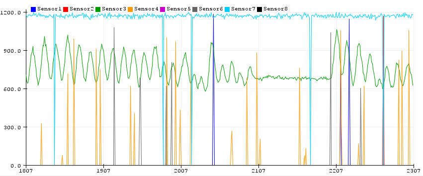
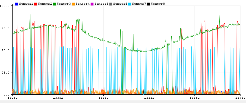
Testing the two arrays side by side, you can see some clear differences in the data below as I move a target (my head ;-)) towards and away from the arrays.
First, you can see that the ultrasonic array samples much faster, so one sequence of me moving my head closer and further takes up the whole screen, as it scrolls faster than the ToF lidar display below it, where I can do it dozens of times in the time it takes the data to scroll off the screen
Sonar/ultrasonic arrayToF Lidar Array
Second, you can see that the Sonar data is noisier. Most of the spurious readings in the ToF Lidar graph (ie, not the green line, which was the sensor pointed right at me) are from the sensor next to it (yellow), which makes sense since the sensors all have a beam spread that could have easily overlapped with the main sensor pointed at me.
That’s true for the sonar data, too (the red line is the sensor right next to the green line of the one pointed at me), but note how the green line, which should be constantly reporting my distance, quite often drops to zero. The blue line, which is a sensor on the other side of the array, is probably seeing a wall that isn’t moving that’s right at the limits of its range, which is why it drops in and out.
So what can we conclude from all this?
ToF Lidar data is less noisy than sonar data
ToF Lidar sensors are slower than sonar sensors
ToF Lidar sensors are more expensive than sonar sensors
Both ToF Lidar and Sonar 1D depth sensors in an array have worse resolution, range and accuracy than 2D Lidar sensors
I’m not sure why I even tried this experiment, since 2D Lidars are great, cheap and easily available 😉
Is there any way to make such an array useful? Well, not the way I did it, unless you’re super keen not to use a 2D mechanical spinning lidar and a RaspberryPi or other Linux computer.
However, it is interesting to think about what a dense array of the ToF chips on a flexible PCB would allow. The chips themselves are about $5 each in volume, and you don’t need much supporting circuitry for power and I2C, most of which could be shared with all the sensors rather than repeated on each breakout board as in the case with the Pololus I used. Rather than have a dedicated digital pin for each sensor to put them in reset mode to change their address, you can use an interrupt-driven daisy-chain approach with a single pin, as FuzzyStudio did. And OSHPark, which I use for my PCBs, does flex PCBs, too.
With all that in mind you could create a solid-state depth-sensing surface of any size and shape. Why you would want that I’m not sure, but if you do I hope you will find the preceding useful.
As we integrate depth sensing more into the DIY Robocars leagues, I’ve been using a simple maze as a way to test and refine various sensor and sensor processing techniques. In my last maze-navigating post, I used a Intel RealSense depth camera to navigate my maze. In this one, I’m using a low-cost 2D Lidar, the $99 YDlidar X4, which is very similar to the RPLidar A1M8 (same price, similar performance). This post will show you how to use it and walk through some lessons learned. (Note: this is not a full tutorial, since my setup is pretty unusual. It will, however, help you with common motion control, Lidar threading and motion planning problems.)
First, needless to say, Lidar works great for this task. Maze following with simple walls like my setup is a pretty easy task, and there are many ways to solve it. But the purpose of this exercise was to set up some more complex robotics building blocks that often trip folks up, so I’ll drill down on some of the non-obvious things that took me a while to work out.
Hardware
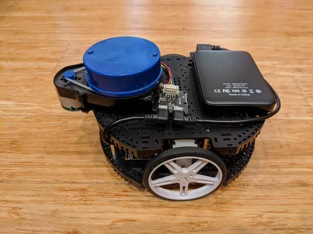
First, my setup: I used a Pololu Romi chassis with motor encoders and a Romi32U control board. Two expansion plates on the top provide a surface for the Lidar. The 32U control board mounts a RaspberryPi 3, which is what we’ll use for most of the processing. Just mount the Lidar on the top, as I have in the picture above, and power it with a separate USB battery (any cheap phone charging battery will work) since the RaspberryPi USB port won’t provide enough power.
Software
The below is a description of some hard things I had to figure out, but if you just want to go straight to the Python code, it’s here.
1) Closed-loop motor control. Although there are lots of rover chassis with perfectly good motors, I’m a bit of a stickler for closed-loop motor control using encoders. That way you can ensure that a rover goes where you tell it to, even with motors that don’t perform exactly alike. This is always a hassle to set up on a new platform, with all sorts of odometry and PID loop tuning to get right. Ideally, the Romi should be perfect for this because it has encoders and a control board (which runs an Arduino-like microprocessor) to read them. But although Pololu has done a pretty good job with its drivers, it hasn’t really provide a complete closed-loop driving solution that works with Python on the on-board RaspberryPi.
Fortunately, I found the RomiPi library that adds proper motion control to the Romi, so if you say turn 10 degrees to the left it actually does that and when you say go straight it’s actually straight. Although it’s designed to work with ROS, the basic frameworks works fine with any Python program. There is one program that you load on the Romi’s Arduino low-level motor controller board and then a Python library that you use on the RaspberryPi. The examples show you how to use it. (One hassle I had to overcome is that it was written for Python 2 and everything else I use needs Python 3, but I ported it to Python 3 and submitted a pull request to incorporate those changes, which was accepted, so if you download it now it will work fine with Python 3)
2) Multitasking with Lidar reading. Reading the YDLidar in Python is pretty easy, thanks to the excellent open source PyLidar3 library. However, you’ll find that your Python code pauses every time the library polls the sensor, which means that your rover’s movements will be jerky. I tried a number of ways to thread or multitask the Lidar and the motor parts of my code, including Asyncio and Multiprocessing, but in the end the only thing that worked properly for me was Python’s native Threading, which you can see demonstrated in PyLidar3’s plotting example.
In short, it’s incredibly easy:
Just import threading at the top of your Python program:
import threading
And then call your motor control routine (mine is called “drive”) like this:
threading.Thread(target=drive).start()
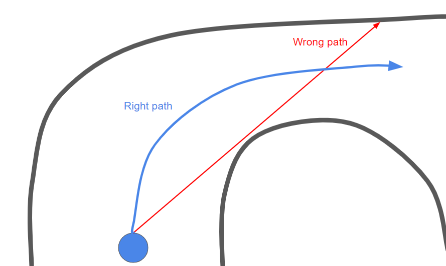
3) Sampling strategies. I totally overthought this one. I tried all sorts of things, from trying to average all the distance points in the Lidar’s 360 degree arc to just trying to find the longest free distance and heading in that way. All too noisy.
I tried batching groups of ten degrees and doing it that way: still too noisy, with all sorts of edge cases throughout the maze. The problem is that you don’t actually want to steer towards the longest free path, because that means that you’ll hit the edge of the corner right next to the longest free path, like this:
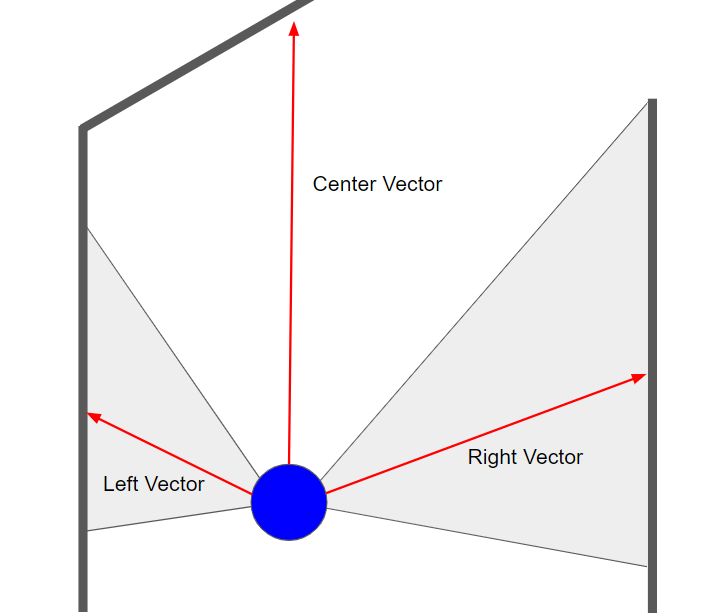
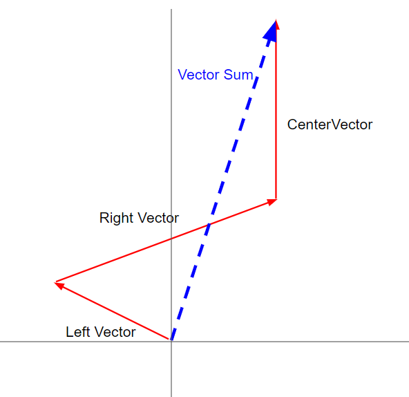
Instead, the best strategy turned out to just keep it simple: define a left side (say 20 to 100 degrees, if straight ahead is 0 degrees), a right side (260 to 340 degrees) and a center (340 to 20 degrees). Get an average distance (vector) for each, like this:
Now that you have three vectors, you can sum them and get the net vector like this (I halve the center vector because avoiding the walls to right and left is more important than seeking some distant free space):
If you set the right and left angles to 45 degrees (pi/4 in radians, which is what Python uses), you can decompose the x and y average values of each zone and add them together like this: